

This page documents the MegaPipe processing of the CFIS dataset. Documentation for using the catalog service is available here and the documentation for the image search tool and cutout service is available here.
The data reduction process starts with the raw images from CFHT. They are detrended with Pitcairn, which performs much the same tasks as Elixir. The bias is removed and the images are flat-fielded. The flat fields are generated from night sky flats for the r-band; the u-band flats are built with traditional twilight flats. The images are astrometrically calibrated using GAIA as reference frame. The photometric calibration is done using PS1 (r-band) and the SDSS to generate a run-by-run differential calibration and an image-by-image absolute calbration. Due to problems with the SDSS, the u-band also requires an ubercal/boot-strapping step. The images are stacked onto 0.5 x 0.5 degree tiles. Catalogs are generated from those tiles and cross matched to the GAIA, PS1 and SDSS.
The data reduction process starts with the raw images from CFHT. They are detrended with Pitcairn, which performs much the same tasks as Elixir. The overscan value is removed as usual. The bias is computed once a semester. The flat fields are generated once per dark run. For the r-band the flat fields are generated using the images themselves. Typically, there are several hundred r-band images taken in a run. The 100 longest exposures are combined using a median to produce a night sky flat. This approach was used in processing the data from the OSSOS survey and was shown to produce slightly (1-2%) deeper output images than using twilight flats. The u-band images however do not contain enough sky photons to generate a satisfactory flat; twilight flats are used.
The AstroGwyn astrometric calibration pipeline is run on the images. The first step is to run SExtractor on each image. The parameters are set so as to extract only the most reliable objects (5 sigma detections in at least 5 pixels). This catalogue is further cleaned of cosmic rays and extended objects. This leaves only real objects with well defined centres: stars and (to some degree) compact galaxies.
This observed catalogue is matched to the astrometric reference catalogue. The (x,y) coordinates of the observed catalogue are converted to (RA, Dec) using the initial WCS provided by CFHT. The catalogues are shifted in RA and Dec with respect to one another until the best match between the two catalogues is found. If there is no good match for a particular CCD (for example when the initial WCS is erroneous), its WCS is replaced with a default WCS and the matching procedure is restarted. Once the matching is complete, the astrometric fitting can begin. Typically 20 to 50 sources per CCD are found with this initial matching.
The higher order terms are determined on the scale of the entire mosaic. That is to say, the distortion of the entire focal plane is measured. This distortion is well described by a polynomial with second and fourth order terms in radius measured from the centre of the mosaic. The distortion appears to be stable over time, even when some of the MegaPrime optics are flipped. Determining the distortion in this way means that only 2 parameters need to be determined (the coefficients of r2 and r4) with typically (20-50 stars per chip) * (40 chips) =~ 1000 observations. If the analysis is done chip-by-chip, a third order solution requires (20 parameters per chip)*(40 chips)= 800 parameters. This can lead to over fitting and is less satisfactory.
The reference catalog is GAIA DR1. The positions of the reference sources were not corrected for mean proper motion, but since the CFHT observation were roughly coeval with the GAIA observations, this is unlikely to introduce much of an error. GAIA DR2 was released recently and will be used for the next round of data processing.
The images are astrometrically calibrated completelely independently from each other. By comparing the positions of stars in overlapping images, the astrometric calibration is estimated to be good to 20 mas in each coordinated, as illustrated in the figures below
The differential photometric calibration (the variation of the zero-point across the focal plane) is measured for each run. The stars in the images are cross matched to an external catalogue (SDSS for the u, Pan-STARRS for the r). The external catalogues are converted into the MegaCam photometric system using the transformations described on the MegaCam filters page. The relevant transformation are reproduced here:
The r-band transformation is a tight fit from Pan-STARRS. The u-band transformation is shows consderably more scatter relative to the SDSS. The adopted u-band transformation is only valid redwards of u-g>1.
The mean zero-point across the image is computed and the deviations relative to this average are mapped as function of CCD and position (x,y) within each CCD. The deviations are agregated on a grid of 4x9 super-pixels and the median deviation is computed. Generally, there zero-point offsets follow a consistent pattern from run-to-run, but there some evolution over time. In a typical run, there will be several hundred images taken in each band. A few runs have a smaller number of images; in these runs there may be not enough images to produce an accurate mapping of the zero-point variation. For these runs, the two neighbouring runs (previous and following) are averaged to produce a map for the affected run. The animated gifs below show the differential photometric gradients across the mosaic in the two bands.
These zero-point variations are removed by expanding the 9x4 super pixels to the original resolution of the CCDs, converting the zero-point difference (which is in magnitudes) to a flux ratio and multiplying each image by the result. The differential zero-point is then remeasured on the corrected CFIS images and examined for large variations. The residuals are plotted as animated gifs below. Generally, the correction is good to 1 mmag, with exceptions on certain runs and certain CCDs on the order of 0.005 mags in r and 0.01 mags in u.
Once the differentiale photometric correction has been applied, a zero-point must be determined for the image as a whole.
For the r-band, the zero-point is determined by transforming the Pan-STARRS photometry into the MegaCam system as before to set up a set of in-field standards. Typically, a few thousand stars are used to set the zero-point. The r-band Pan-STARRS to MegaCam transformation is robust, the Pan-STARRS photometry is uniformally excellent, and Pan-STARRS covers the entire CFIS area. The r-band zero-points are correspondingly accurate, good to about 0.005 magnitudes.
For the u-band, the transfomation from the SDSS to MegaCam is not as clean. CFIS covers some fields which not covered, or only partially covered by the SDSS. Further, the SDSS photometry in the u-band has some problems as illustrated below:
These problems mean that the simple approach used for the r-band is insufficient. Instead, a boot-strapping/ubercal process is required. Initial zero-points are computed using either the SDSS as in-field standard where possible. The zero-points of these images are use to compute nightly zero-points which are used to set initial zero-points of the images not on the SDSS. The boot-strapping process starts by flagging all images directly calibrated with the SDSS, and all images taken on photometric nights as PHOT. The rest are set to NOT_PHOT. Catalogs derived from all the images are cross matched, and the zero-point differences between all the images is computed. There follows a set of iterations. In each iteration, the first step is to check for consistency. If the zero-point difference between two images flagged as PHOT is found to be greater than 0.02 mags, they are reset to NOT_PHOT. The second step in each iteration is to attempt to calibrate the NOT_PHOT images using the zero-points of the overlapping PHOT images. If at least 3 PHOT images overlap a NON_PHOT image, and the zero-points transfered to the new images are consistent within 0.01 magnitudes, the zero-point of the image in question is set to that value, then the image is now flagged as PHOT, and can now be used to calibrate neighboring NOT_PHOT images in the next iteration. Eventually, most of the images can calibrated. The remaining images usually do not overlap enough PHOT images. A small number of images were taken under conditions where part of the MegaCam mosaic was obscured, presumably by clouds. These images will have different relative zero-points across the field, and will always fail the consistency test. Both classes of NOT_PHOT images have a zero-point to the best available zero-point, either by direct calibration, nightly zero-point or boot strap.
Examining the residuals of this process gives an estimate of the photometric uncertainties. The average zero-point difference is 0.009 magnitudes.
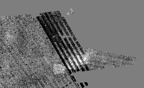
Comparing the CFIS-u data to the SDSS, we can see that most of the major differences between the two surveys follow the observing pattern of the SDSS.
The individual images are available via the graphical search tool
Next the calibrated individual images are stacked. In the past, MegaPipe has stacked on to a pixel grid defined by the input images. Because of the large dithers in the CFIS observing pattern, which causes many overlaps between between neighboring images, this is inpractical. Instead a set of tiles is defined and the images resampled unto these tiles. The tiles are 10000x10000 pixels with a pixel size of 0.1857 arcsecond per pixel, approximately the native resolution of MegaCam. The tiles are spaced exactly 0.5 degrees apart in Dec and 0.5/cos(Dec) apart in RA. The tiles of a small (~3%) overlap. The tiling is best illustrated by going to the graphical search tool, zooming in, and toggling the "Show Images" and "Show Tiles" buttons.
The tiles have names in the format CFIS.xxx.yyy.f.fits. xxx and yyy correspond to the RA, Dec of the tile centres as follows:
xxx=ra*2*cos(dec)
yyy=(dec+90)*2

dec=yyy/2-90
ra=xxx/2/cos(dec)
xxx therefore can run from 0 to 719 (but there will be only 720 tiles around the equator) and yyy runs from 0 to 360, going from pole to pole.
Each tile is created independently of its neighbors. The relevant individual calibrated images are retrieved. Swarp is used to resample the images according to the astrometric calibration and scale the images according to the photometric calibration. The resampled image are combined with a median combine. The swarp configuration file is cfis.swarp.
The average IQ is computed for each image. Because many different images will combined into one tile in a varied pattern, this value may not be representative of every part of the tile. Similarly, the magnitude limits may not be representative. The magnitude limits are computed by adding fake objects to the tiles to determine the 50% completeness limit and by measuring both the 5-sigma point source 2-arcsecond aperture limit, and the 5-sigma MAG_AUTO limit.
The tiles are available via the graphical search tool
The final step is to generate catalogs. SExtractor on the u-band and r-band images separately. The SExtractor configuration file is cfis.sex. Most of the parameters in the output catalog are used as is. The only exception is the aperture magnitude, which has a small aperture correction applied. Note that, because of the large dithers, the point source FWHM can vary strongly over the field. No single aperture correction is appropriate for a tile. Therefore, each source, the position is traced back to the original input images and a predicted FWHM is computed. This FWHM is used to produce an aperture correction. In the catalogs, the FWHM is recorded as u_IQ and r_IQ, and the aperture correction is recorded as u_APPCOR and r_APPCOR.
The u- and r-band catalogs are cross matched. The common objects are identified and their catalog entries are merged. Because CFIS is relatively shallow, the image quality generally excellent and the astrometry very good, the chance of spurious matches is quite low. The machinery used for the CFHTLS (see this page) was not necessary.
The u+r merged catalog was in turn cross-matched with the following catalogs:
The final merged catalog is available via the Query tool.