This release contains all data taken before January 2021, including ~7000 square degrees of u-band data and ~3600 square degrees of r-band data. The u-band photometric calibration method now uses Pan-STARRS 3PI (PS-3pi) and GALEX, greatly improving its reliability. LSB (Low Surface Brightness) stacks are now available for the r-band images. The catalog generation has been improved. The data are available on CANFAR through the following links:
You can use your browser, or standard tools like curl and wget to retrieve the data, however the best way is the VOspace python tool, available here.
The data reduction process starts with the raw images from CFHT. They are detrended with Pitcairn, which performs much the same tasks as Elixir. The bias is removed and the images are flat-fielded. The flat fields are generated from night sky flats for the r-band; the u-band flats are built with traditional twilight flats. The images are astrometrically calibrated using Gaia as reference frame. The photometric calibration is done using PS-3pi (r-band) and a combination of the SDSS, PS-3pi and GALEX to generate a run-by-run differential calibration and an image-by-image absolute calibration. The individual images are stacked onto 0.5 x 0.5 degree tiles. Catalogs are generated from those tiles. The catalogs are split into patches such that the area of each patch is covered by a single set of input images, and therefore have homogeneous depth and image quality properties. The patch catalogs are processed separately then merged back into tile catalogs.
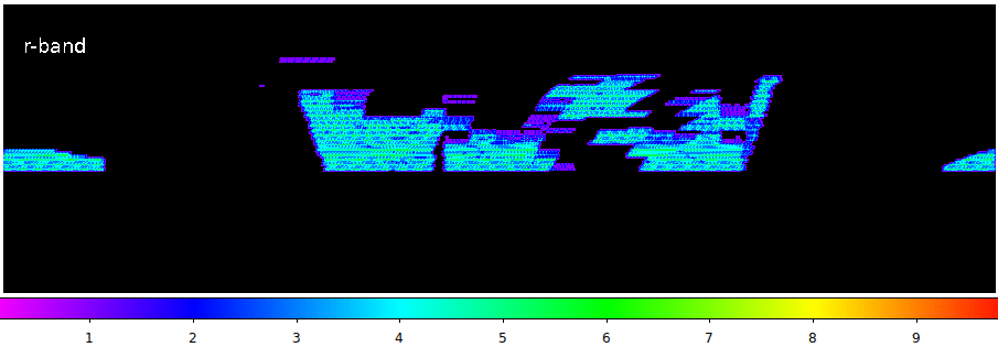
The following two plots show the coverage for CFIS DR3 and u and r, indicate the number of images covering each part of the sky.
The CFIS DR3 is based on all data acquired before January 2021. Images with bad seeing and trailed images were rejected. All images were classified by machine learning algorithm. In addition a significant fraction of the images were visually inspected, including all the images rejected by machine learning algorithm. In several cases (amounting to about 5% of the images) there were redundant images; the same pointing was observed multiple times. For the r-band, only the best available image was included in the processing. For the u-band, all the images were retained. 54 of the images could not be successfully calibrated, either due holes in the Gaia reference catalogue, or because of difficulties in the u-band calibration (see the photometry section below). The following table summarizes the image selection:
| u | r | |
| Total number of images | 23971 | 11995 |
| Accepted images | 23166 | 9444 |
| FWHM cut | 1.5 arcsec | 1 arcsec |
| Ellipticity cut | 0.15 | 0.10 |
| Median seeing | 0.89 | 0.69 |
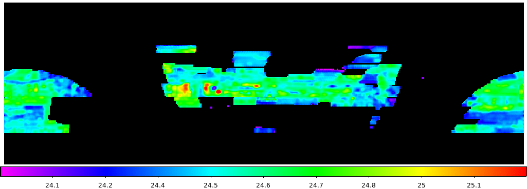
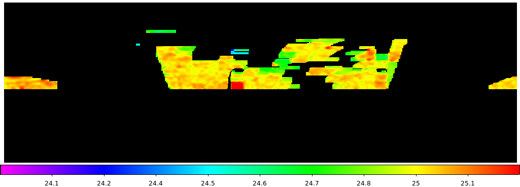
| Median depth (point source, 5-sigma,2 arcsec) | 24.6 | 25.0 |
| Area | 6200 sq deg | 2800sq deg |
| Number of tiles | 28325 | 14576 |
| Number of patches | 821103 | 279681 |
| Number of sources | 272606064 | 451728248 |
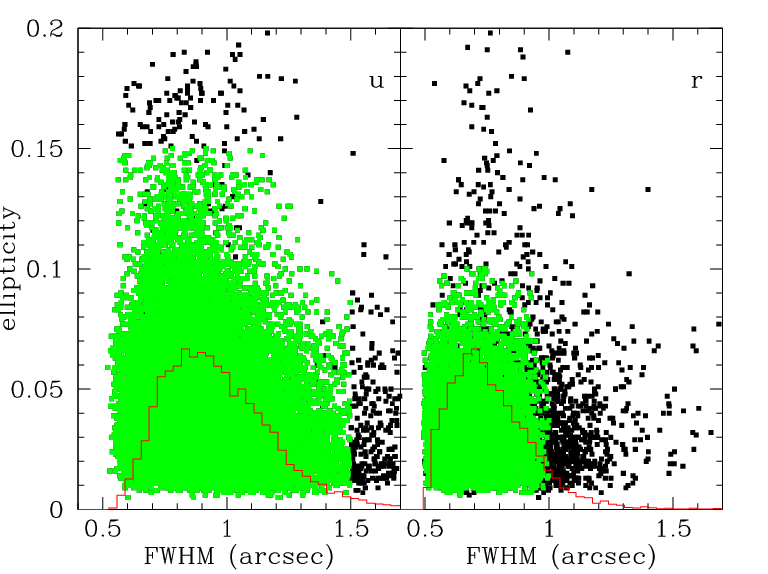
The figure below shows the FWHM and ellipticity of the CFIS image.
The following tables give the list of CFIS input images. The last column contains either "OK" (meaning the image was included in DR3) or the reason for rejection.
Versions of the above plots in FITS format at scale of 0.1 degree per pixel, which can be used to determine coverage are available from the links below:
The data reduction process starts with the raw images from CFHT. They are detrended with Pitcairn, which performs much the same tasks as Elixir. The overscan value is removed as usual. The bias is computed once a semester. The flat fields are generated once per dark run. For the r-band the flat fields are generated using the night-time science images themselves. Typically, there are several hundred r-band images taken in a run. The 100 longest exposures are combined using a median to produce a night sky flat. This approach was used in processing the data from the OSSOS survey and was shown to produce slightly (1-2%) deeper output images than using twilight flats. The u-band images however do not contain enough sky photons to generate a satisfactory flat; twilight flats are used.
The AstroGwyn astrometric calibration pipeline is run on the images. The first step is to run SExtractor on each image. The parameters are set so as to extract only the most reliable objects (5 sigma detections in at least 5 contiguous pixels). This catalogue is further cleaned of cosmic rays and extended objects. This leaves only real objects with well defined centres: stars and (to some degree) compact galaxies.
This observed catalogue is matched to the astrometric reference catalogue. The (x,y) coordinates of the observed catalogue are converted to (RA, Dec) using the initial WCS provided by CFHT. The catalogues are shifted in RA and Dec with respect to one another until the best match between the two catalogues is found. If there is no good match for a particular CCD (for example when the initial WCS is erroneous), its WCS is replaced with a default WCS and the matching procedure is restarted. Once the matching is complete, the astrometric fitting can begin. Typically 20 to 50 sources per CCD are found with this initial matching.
The higher order terms are determined on the scale of the entire mosaic. That is to say, the distortion of the entire focal plane is measured. This distortion is well described by a polynomial with second and fourth order terms in radius measured from the centre of the mosaic. The distortion appears to be stable over time. Determining the distortion in this way means that only 2 parameters need to be determined (the coefficients of r2 and r4) with typically (20-50 stars per chip)x(40 chips) =~ 1000 observations. If the analysis is done chip-by-chip, a third order solution requires (20 parameters per chip)x(40 chips)= 800 parameters. This can lead to over fitting and is less satisfactory.
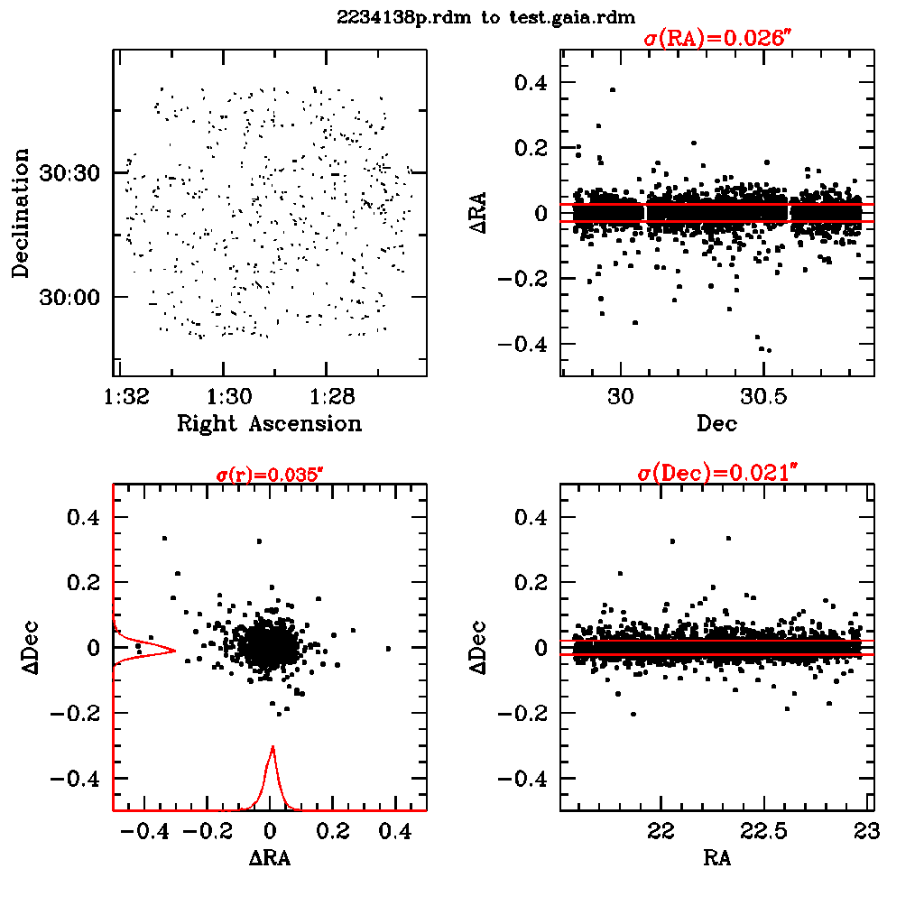
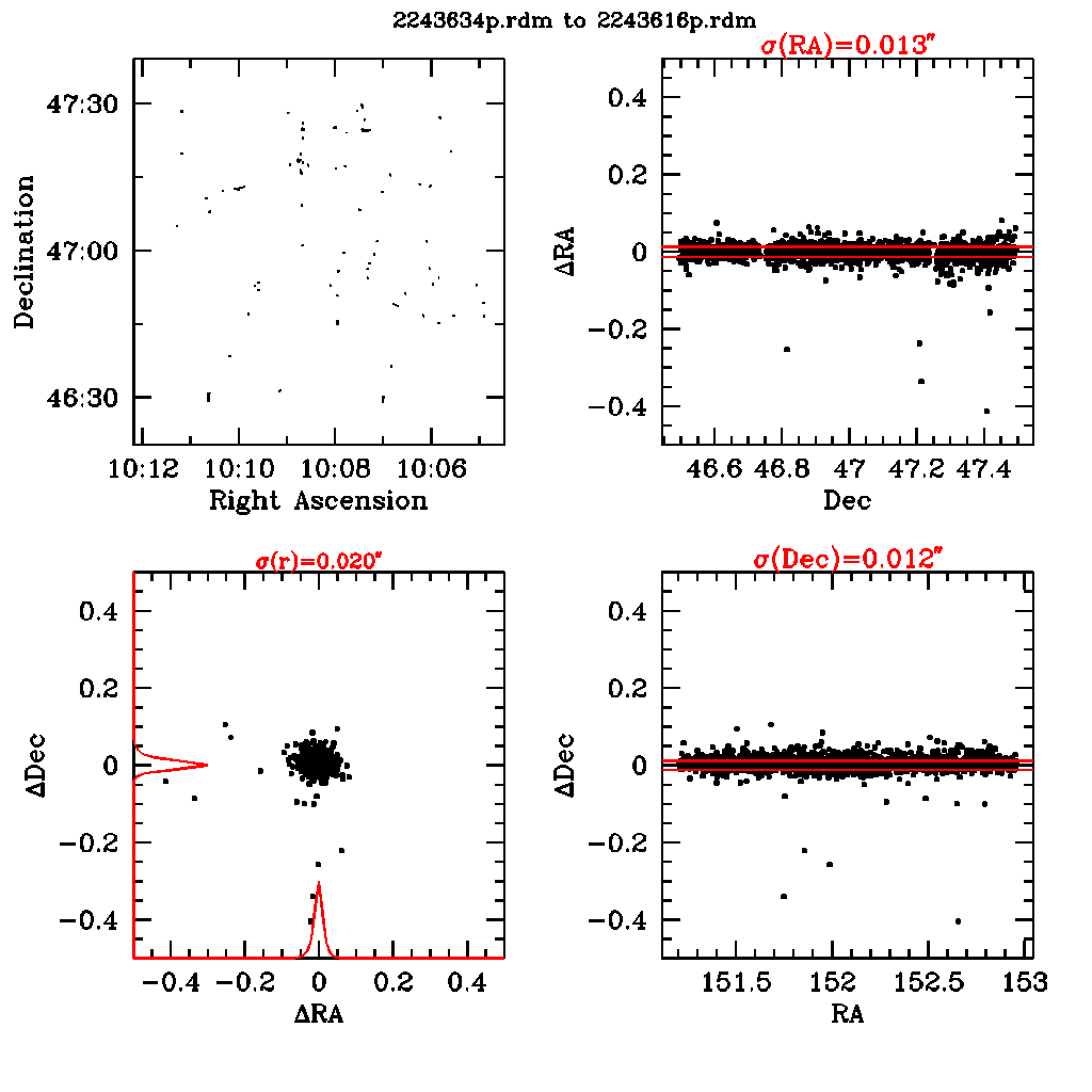
The reference catalog is Gaia EDR3. The positions of the reference sources are corrected for proper motion. The images are astrometrically calibrated completely independently from each other. By comparing the positions of stars in overlapping images, the astrometric calibration is estimated to be good to 20 mas in each coordinate, as illustrated in the figures below:
The differential photometric calibration (the variation of the zero-point across the focal plane) is measured for each run. The stars in the images are cross matched to an external catalogue (SDSS for the u, Pan-STARRS for the r). The external catalogues are converted into the MegaCam photometric system using the transformations described on the MegaCam filters page. The relevant transformations are reproduced here:
The r-band transformation is a tight fit from Pan-STARRS. The u-band transformation shows considerably more scatter relative to SDSS. The adopted u-band transformation is only valid redwards of u-g>1.
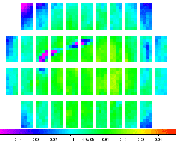
The mean zero-point across the image is computed and the deviations relative to this average are mapped as function of CCD and position (x,y) within each CCD. The deviations are aggregated on a grid of 4x9 super-pixels and the median deviation is computed. Generally, the zero-point offsets follow a consistent pattern from run-to-run, but there some evolution over time. In a typical run, there will be several hundred images taken in each band. A few runs have a smaller number of images; in these runs there may be not enough images to produce an accurate mapping of the zero-point variation. For these runs, the two neighbouring runs (previous and following) are averaged to produce a map for the affected run. The animated GIFs below show the differential photometric gradients across the mosaic in the two bands.
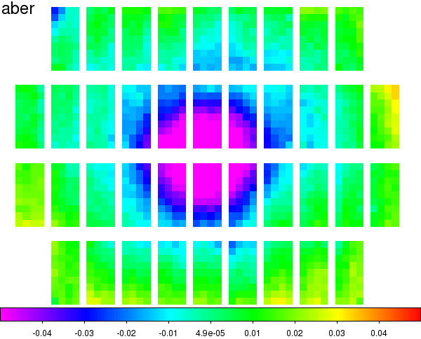
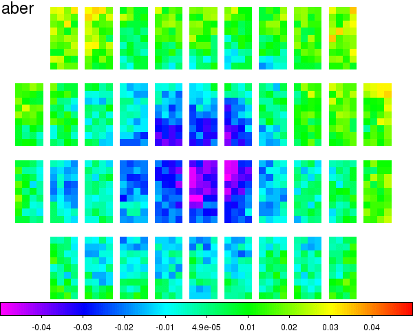
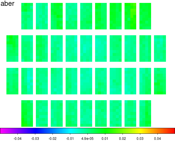
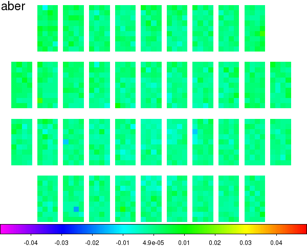
These zero-point variations are removed by expanding the 9x4 super pixels to the original resolution of the CCDs, converting the zero-point difference (which is in magnitude) to a flux ratio and multiplying each image by the result. The differential zero-point is then remeasured on the corrected CFIS images and examined for large variations. The residuals are plotted as animated GIFs below. Generally, the correction is good to 1 mmag. (0.1%), with exceptions on certain runs and certain CCDs on the order of 5 mmag. in r and 10 mmag. in u (1%).
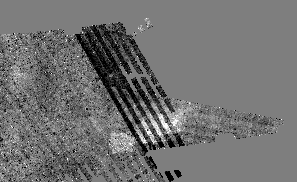
For 3 runs in 2019, there was a significant change to the photometric pattern. There was a blob of lower sensitivity covering multiple chips, as illustrated below. The nature of this blob is not exactly clear, although it disappeared when the dewar window was cleaned:
Once the differential photometric correction has been applied, an absolute zero-point must be determined for the image as a whole. For the r-band, the zero-point is determined by transforming the Pan-STARRS photometry into the MegaCam system as before to set up a set of in-field standards. Typically, a few thousand stars are used to set the zero-point. The r-band Pan-STARRS to MegaCam transformation is robust, the Pan-STARRS photometry is uniformly excellent, and Pan-STARRS covers the entire CFIS area. The r-band zero-points are correspondingly accurate, good to about 0.005 magnitudes (0.5% photometry).
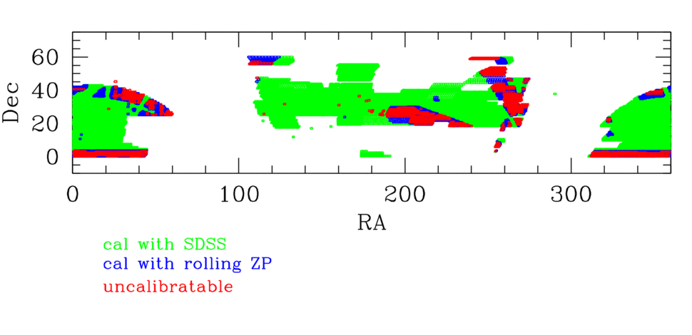
For the u-band, the transformation from the SDSS to MegaCam is not as clean. CFIS covers some fields which not covered, or only partially covered by the SDSS. Further, the SDSS photometry in the u-band has some problems as illustrated below:
The first attempt to solve this problem used the good parts of the SDSS to compute zero-points over the course of photometric nights. The zero-points were computed using all usual images taken within an hour of the exposure to be calibrated. This rolling zero-point method increased the number of images that could be calibrated, but because not all the nights were photometric, and because of the observing pattern used, a significant fraction of the u-band data could not be calibrated, as illustrated below.
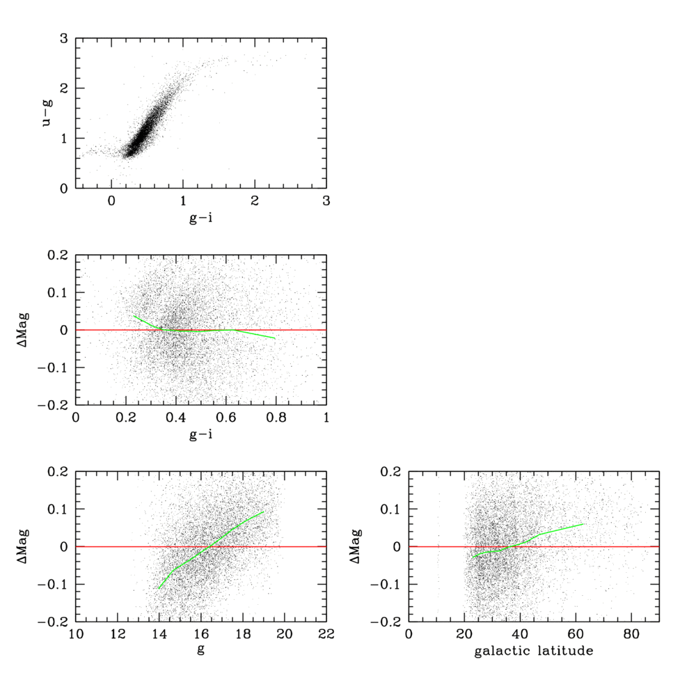
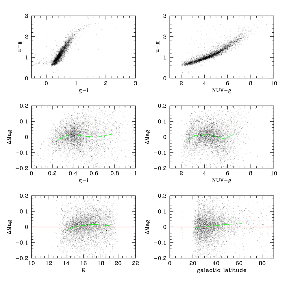
Attempts have been made to use Pan-STARRS to calibrate u-band in the past (see Finkbeiner et al. 2016), but ultimately the strong metallicity dependence of the u-g colour makes this infeasible, as illustrated in the figure below. The top panel shows the colour-colour diagram u-g vs. g-i. If a 5-th order polynomial is fitted to this figure, one can produce a predicted u magnitude. The residuals of this fit are plotted in the next set of figures, against g-i, g, and galactic latitude. Halo stars being more metal-poor, at high galactic latitudes and greater distances the stars will typically be bluer. This shows up in the bottom two panels of the figure below.
However, with information from the NUV channel of GALEX the picture changes significantly: The figure below shows the same residuals as before, but this time including a 5-th order polynomial fit in NUV-g. The gradients in the bottom two panels is much smaller.
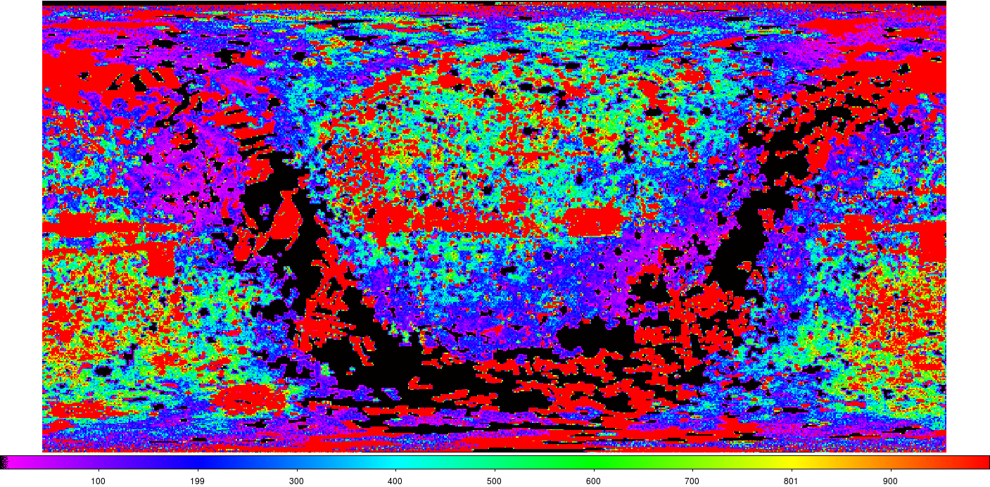
GALEX coverage is fairly extensive, but ubiquitous, as shown in the figure below, which shows the source density per square degree across the sky.
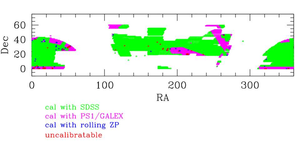
In the end, while almost all the CFIS u-data can be calibrated, a total 56 u-band images were observed parts of the sky where the SDSS was unreliable, and there were an insufficient number of GALEX sources and either the night was not photometric or no reliable zero-point could be calculated, as shown in the map below. While annoying, this represents a tiny fraction of the 21412 u-band images (0.2%).
The individual calibrated images can be found in https://www.canfar.net/storage/list/cfis/pitcairn. Each image has an updated header with astrometric calibration expressed in usual CRVAL/CRPIX/CD keywords, plus PV keywords to express distortion. The photometric zero-point is uniform across the image. The PHOTZP keyword gives the zero-point. This zero-point includes exposure time and airmass corrections.
Next the calibrated individual images are stacked on a set of tiles. The tiles are 10000x10000 pixels with a pixel size of 0.1857 arcsecond per pixel, approximately the native resolution of MegaCam (0.187). The tiles are spaced exactly 0.5 degrees apart in declination and 0.5/cos(Dec) apart in right ascension. The tiles feature a small (~3% total) overlap. The tiling is best illustrated by going to the graphical search tool, zooming in, and toggling the "Show Images" and "Show Tiles" buttons.
The tiles have names in the format CFIS.xxx.yyy.f.fits. xxx and yyy correspond to the RA, Dec of the tile centres as follows:
xxx=ra*2*cos(dec)
yyy=(dec+90)*2

dec=yyy/2-90
ra=xxx/2/cos(dec)
xxx therefore can run from 0 to 719 (but there will be 720 tiles only around the equator) and yyy runs from 0 to 360, going from pole to pole.
WeightWatcher is run on each input image. WeightWatcher masks out bad columns and does a fairly good job of masking cosmic rays.
Each tile is created independently of its neighbors. The relevant individual calibrated images are retrieved. SWarp is used to resample the images according to the astrometric calibration and scale the images according to the photometric calibration. The resampled image are combined with a weighted mean combine, using the WeightWatcher weight maps. The SWarp configuration file is cfis.swarp.
The tiles and the corresponding weight maps can be found in https://www.canfar.net/storage/list/cfis/tiles_DR3. The zero-point of the tiles is 30.000. While the tiles FITS headers contain keywords indicating depths and IQ values, these numbers are the mean over the tile and are unlikely to be representative of any particular part of the tile (see the discussion in the section below). Similarly the effective gain changes across each tile.
The CFIS-r is now offered with the low surface brightness signal recovered through a complete LSB run at CADC: the input images are the individual calibrated images described above (the LSB enabled images feature the same level of astrometric and photometric accuracy). Following a rejection/validation process, only LSB valid individual images are offered and included in the LSB stacks/tiles for CFIS-r tiles at full depth only (3 visits).
The properties and performance of the CFIS-r DR3 LSB dataset are presented on this UNIONS note.
The LSB stacking follows the same procedure as the regular MegaPipe stacks except for single a pedestal removal from the entire image in SWarp (versus its internal 2D background subtraction). Due to residual gradients caused by the very bright stars found in our footprint (V < 6th mag.), some stacks will suffer from residual background tilts (c.f. the LSB documentation listed above): for any point source science we recommend the adoption of the regular MegaPipe stacks.
The individual LSB corrected images can found in at:https://www.canfar.net/storage/list/cfis/lsb_individual
The LSB tiles can be found at: https://www.canfar.net/storage/list/cfis/tiles_LSB_DR3
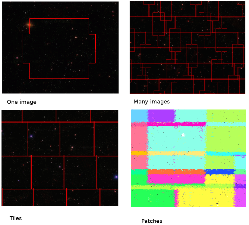
The final step is to generate catalogs. This is greatly complicated by the way the data was acquired, with multiple images, with different seeing and depths partially overlapping each other across the sky. This problem is solved with a software package called PTOUSE = Parallel Tessellated Optimal Uniform Source Extraction.
Some definitions:
These different areas are illustrated below:
The photometric calibration of the individual images is done using an aperture that works out to the equivalent to SExtractor's MAG_AUTO for stars. This aperture works out to 5.15 times the IQ. Internally, this magnitude is called MAG_PERF. While robust, this aperture is quite large, which means it is not optimal for faint sources, although it is adequate for the bright stars that are used for calibration.
The catalog generation is done with a software package called PTOUSE = Parallel Tessellated Optimal Uniform Source Extraction. PTOUSE runs SExtractor on each tile, with 20 closely spaced fixed apertures. Each detected source on the tile is traced back to the relevant input images. This list of images defines a patch.
The next step loops over the patches. Using the closely spaced apertures, PTOUSE maps out the curve of growth. Using the flux in the inner apertures, PTOUSE extrapolates out to the MAG_PERF aperture. This extrapolation depends on IQ of course which is why it is done at the patch level, where the IQ is homogeneous. For some patches, there are not enough stars to measure the curve of growth. However, it turns out the radial PSF of MegaCam can be described to fairly high accuracy with a single curve, scaled to the seeing. See the figure below.
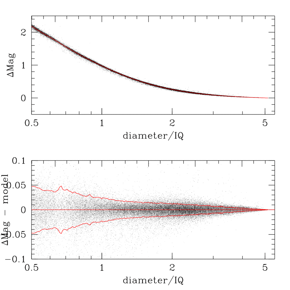
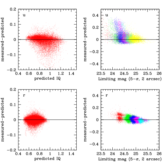
Even if there are not enough stars to measure the IQ, the IQ of a patch can be predicted from the IQ of its input images, typically to within 0.02 arcsec. Because the coaddition was done using a weighted mean, the IQ of each patch is very close to the mean of the IQs of the input image, as shown below.
Thus MAG_COG is a robust and consistent measure of flux for point sources despite the changes in IQ across the survey. Because MAG_COG is measured through a set of relatively small apertures, it's relatively low noise. Because it's measured in multiple apertures, there some robustness (not perfect) against any cosmic rays that slipped through the cosmic rejection step.
The limiting magnitude is also measured at the patch level, since it depends heavily on the number and depth of the input images. Again, if there are not enough stars to properly measure the depth in a given patch, it can be robustly predicted from the depths of the input images.
In the last step, PTOUSE aggregates the patches back to the tiles. Separate from the catalogues, there are tables for each tile where each source is mapped back to the input images, down the chip and x,y coordinates within that chip. The tiles overlap slightly: stars in the overlap regions are trimmed out. The u and r catalogs are merged by requiring a positional match between sources of less than 0.5 arcseconds, with an additional criteria, to avoid confusion, that there can be no second source within 0.5 arcseconds. Because CFIS is relatively shallow, the image quality generally excellent and the astrometry very good, the chance of spurious matches is quite low. The machinery used for the CFHTLS (see this page) was not necessary.
The catalos can be queries via the CADC TAP service with the UNIONS catalog query page. The catalogs can be found in ASCII format at: https://www.canfar.net/storage/list/cfis/catalogs_DR3.
The catalogs are split by tile. There are 3 sets of catalogs: separate u- and r-band catalogs (u.cat and r.cat) and a merged catalog (.cat). There are 20 values for aperture photometry. The diameters in MegaCam pixels are: 1,2,3,4,5,6,7,8,9,10,12,14,16,18,20,22,25,30,35,40. FLUX_RADIUS is the half-light radius. Most of the column names are standard SExtractor parameters; the exceptions are listed below:
# 60 MAG_APAUTO     Aperture magnitudecorresponding to MAG_AUTO for star      [mag]
# 61 MAGERR_APAUTO  RMS error for MAG_APAUTO                                  [mag]
# 62 MAG_COG        Curve of growth magnitude                                 [mag]
# 63 MAGERR_COG     RMS error for MAG_COG                                     [mag]
# 64 MAG_2ARC       Aperture magnitude in a 2 arsecond aperture               [mag]
# 65 MAGERR_2ARC    RMS error on MAG_2ARC                                     [mag]
# 66 IQ             Seeing                                                 [arcsec]
# 67 MAGLIM_2ARC    5-sigma point source limiting magnitude for MAG_2ARC      [mag]
# 68 MAGLIM_APAUTO  5-sigma point source limiting magnitude for MAG_APAUTO    [mag]
# 69 MAGLIM_COG     5-sigma point source limiting magnitude for MAG_COG       [mag]
MAG_COG (described above) is optimized for stars. MAG_AUTO is optimal for galaxies. Note that the limiting magnitude and IQ can vary significantly across the CFIS survey. Therefore every source has an IQ and 3 limiting magnitudes associated with it.
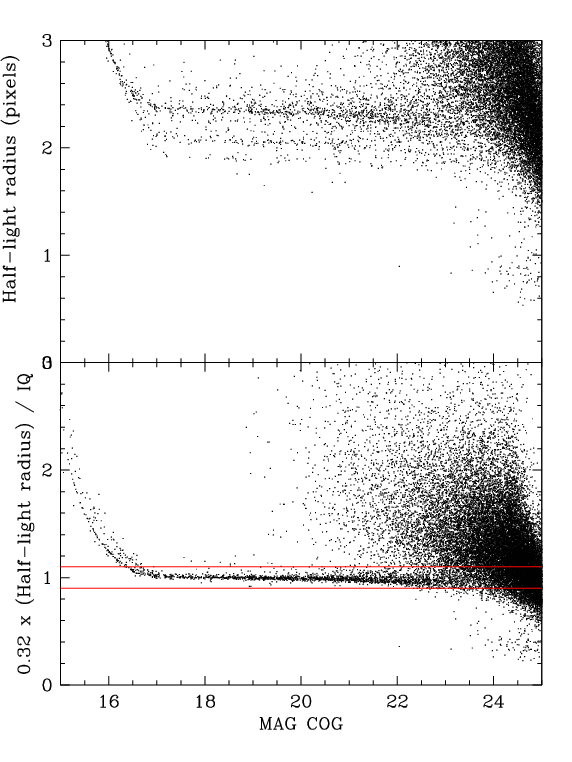
Several attempts at star/galaxy separation algorithms were made. While fine at the bright end, all are prone to confusion at the faint end. Ultimately some machine learning or forced photometry method will be brought to bear on the problem. In the meantime, the following method is satisfactory at magnitudes brighter than 22.5. The top panel of the figure below shows half-light radius (FLUX_RADIUS) as a function of magnitude (MAG_COG) for a tile. There are several horizontal loci, corresponding to stars in the different patches of the tile. If the values of FLUX_RADIUS are divided by the values of IQ (with a factor of 0.32 to convert from FWHM in arcseconds to half-light radius in pixels) the loci collapse into a single locus, centred around 1. Cuts at 0.9 and 1.1 in this parameter neatly contain the stellar locus at the bright end. At the faint end, errors in FLUX_RADIUS, and the increased number of small, compact galaxies cause confusion.
Some analyses may require measurements of the sources on the original images. For this purpose there are set of provenance catalogs in https://www.canfar.net/storage/list/cfis/provenance. These catalogs have 5 columns:
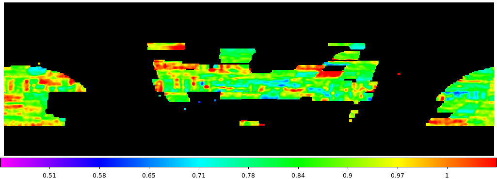
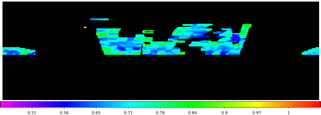
Because of the more stringent requirements on seeing, and because of the use of QSO-SNR observing mode, the r-band depths and IQ are fairly homogeneous. The u-band exposure time on the other hand was fixed at 80 seconds, and the range in seeing conditions was larger, leading to fairly heterogeneous depths. In addition, some pointings were mistakenly re-observed multiple times, leading to greater depths.
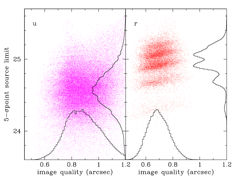
The following images are maps showing the spatial variation of the IQ and depth over the sky.